by Ruth Mottram, DMI

Glaciers and ice sheets are vast slow moving reservoirs of fresh water fed by precipitation, particularly snow fall, and losing mass by melting and calving of icebergs. If more snow falls than is lost to melt or icebergs then the glacier will grow and advance and conversely, if more melts or calves than accumulates it will retreat and shrink. So far, so simple.

An important part of our day to day activities in the research department relates to the effects of climate change in the Arctic and in particular the total mass balance of the Greenland ice sheet. This is important globally and regionally because it determines how much sea level will rise, or fall, it also has local temperature effects and implications for, for example, land use and hydropower developments, and potentially may affect regional and global climate through changes to ocean or atmospheric circulation. 

The total mass balance has two main components, that dealing with surface processes of precipitation, melt and runoff and the dynamic component related to the flow of glaciers, including calving processes. Partitioning mass loss into these two components is important to understand how the ice sheet responds to a climate forcing, for example in the early 2000s, a number of outlet glaciers in south east Greenland accelerated and retreated, leading to a large mass loss by dynamic processes. However, these types of events are usually short lived and over a longer term time scale surface mass losses are considered more important for the Greenland ice sheet. In Antarctica by contrast most of the mass lost is via calving of icebergs or melt occurring from the undersides of floating ice shelves in the ocean. This latter process is also likely to be significant in some parts of Greenland and for example has been related to the massive acceleration and retreat seen in the Jakobshavn glacier in the last 10 years, but it is as yet poorly quantified and modeled.

 The launch in 2013 of the website polarportal.dk (polarportal.org in English, a joint production of DMI, GEUS and DTU-Space) now allows anyone to check the current “health” of the Greenland ice sheet, including glacier front positions for selected outlet glaciers based on satellite image and an estimate based of total mass balance using a product developed from GRACE satellite gravity measurements. The daily surface mass balance (smb) of the ice sheet is also presented and compared with the long term average to indicate what the ice sheet surface mass balance “weather” is doing today. 

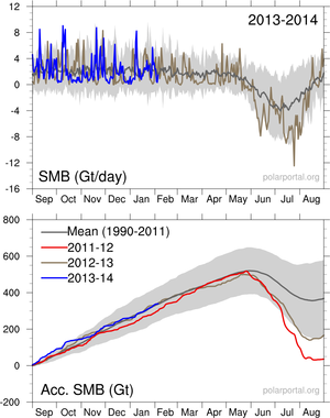The smb model system on the polar portal takes output from the HIRLAM weather forecasting model and runs it through a second smb model each day. This is accumulated over the course of a hydrological year (running from 1st September to 31st August) to give the annual mean smb. On the site it is also compared with the average of a 24 year climate simulation (1989 – 2014) using the HIRHAM5 regional climate model. This model has a slightly different atmospheric forcing but the same surface mass balance model so it allows us to assess how representative the current weather is of the current climate (Figure 1).

The surface mass balance of Greenland is dominated by snow fall as figure 1 shows. Accumulation occurs for 9 months of the year with ablation occurring mostly in the 3 summer months of June, July and August. Our model simulations, which have been successfully validated against ice core observations and precipitation measurements at weather stations both on (PROMICE and GC-NET weather stations) and off the ice (DMI Automatic weather stations) suggest an annual mean of around 664 km3 of snow falls over the ice sheet at the present day (1989 – 2012). These layers are gradually compressed into glacier ice and start to flow downslope in response to the change in surface gradient caused by surface melt at lower elevations and accumulation at higher. Thus surface mass balance drives the internal flow of glaciers.

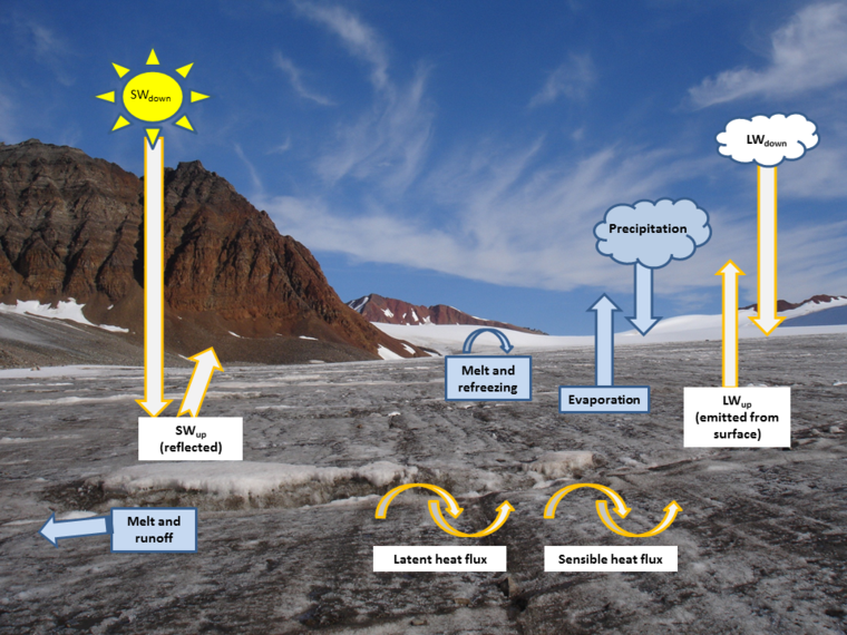
Mass loss processes are the other part of the surface mass balance calculation. Sublimation and evaporation of water vapour direct from the surface is an important mass loss process particularly in winter, but in the summer melt processes dominate mass loss.  Melt is commonly calculated using one of two methods, a temperature index (or “degree day”) model which takes some function of measured or modeled temperature above the melting point and calculates the melt rate from that, or the energy balance approach which is more physically representative of the processes. At DMI our climate model uses the latter technique which involves summing the net radiation and turbulent heat fluxes with the ground heat flux to find the total energy available at the surface (equation 1).

SWnet + LWnet + QE + QL + GE – ME = 0 

The model calculates the incoming solar shortwave radiation and balances by a reflected component dependent on surface albedo to give SWnet and incoming long wave radiation, mainly emitted from the atmosphere and clouds is balanced by the outgoing long wave calculated based on surface emissivity to give the net long wave (LWnet). The net turbulent fluxes in (1) are comprised of the sensible heat flux (QE), which describes the transfer of energy due to the difference in temperature between the surface and the atmosphere (it is effectively sensible heat transfer that gives rise to the wind chill effect for example) and the latent heat term (QL, also known as enthalpy) that is a consequence of phase changes (melting, evaporating, freezing and sublimation) at the surface. These latter two terms are strongly dependent on the air temperature, humidity and wind speeds. The atmospheric energy terms are summed together with the ground heat flux (GE) which includes the energy transfer to and from the subsurface, to give the surface or skin temperature.  The skin is best imagined as an infinitesimally thin layer at the surface, on a glacier we assume that this temperature cannot reach above the melting point and since the first law of thermodynamics applies, any additional energy is available for melt (ME). In our model both snow and glacier ice are allowed to melt and refreeze or run off.

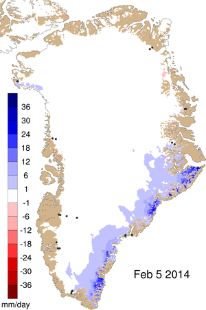
Melt can occur to what may be surprisingly high elevations on the ice sheet. For example, the automatic observation stations of the PROMICE network recorded melt at 1800m altitude near Kangerlussuaq in 2013, a relatively average temperature (compared  to the 1989-2012 mean) summer in Greenland. In 2012 the whole ice sheet was briefly observed to have a surface melt layer and melt was even observed at the Summit station. The unusual conditions in the summer of 2012 focused much attention on the Greenland ice sheet and it was an excellent test case for the model system since both HIRLAM and HIRHAM5 managed to reproduce these extreme conditions (see Figure 2). However, as this event graphically showed melt is not the same thing as mass loss from the ice sheet.

 When surface snow melts or if it rains on to a snow layer, the water first percolates into the lower layers of the snow pack and refreezes, if the snowpack is cold enough, adding mass to the glacier. This is a very heterogenous process and therefore extremely complicated to model with features such as ice lenses and ice fingers observed forming in these lower layers. These ice features have a significant impact on the density of the snowpack, they lower the local albedo when they reach the surface and their formation releases latent heat that warms the surrounding snow. The formation of large ice layers can also prevent further melt water percolation into deeper layers but this refrozen ice may still melt again later in the melt season if it is exposed to the surface, effectively delaying runoff so it is an important process to consider when calculating smb. 

Our final smb calculation is thus (2)

SMB = Precipitation – Evaporation – Sublimation – Runoff  (2)

Where

RUNOFF = Melt + Rainfall - Refreezing

The HIRHAM5 regional climate model estimates that the average annual smb is around 367 km3 over the 1989 – 2012 period which is consistent with other model estimates and with calculated smb at locations where the components are measured accurately. In the future our models project a small increase in precipitation over the interior but much enhanced melt and runoff is expected to more than compensate for this leading to accelerated retreat and sea level rise though the magnitude of this is highly dependent on chosen emissions scenario and to a certain extent on the GCM. 

Combining the smb model with the output from the HIRLAM weather forecast model for Greenland is thus a powerful way of realistically assessing the current state of balance of the Greenland ice sheet and for the first time ever we now have the means to do so in in near real-time.